Introduction

Only 60 new player candidates are drafted annually in the NBA Draft, the entry system for non-professional athletes into the National Basketball Association. Each of the first 30 draft picks has a four-year, fixed salary which scales based on pick position. A hard salary cap, instituted in the most recent Collective Bargaining Agreement between NBA teams and the Players’ Association, introduces strict financial constraints that can come into effect when a team enters negotiations with its drafted player after his initial four-year contract concludes. (Kaplan, 1617) Thus, it has become even more important in recent years to draft players who can produce on-court value requisite to the salary tied to their respective draft positions.

Problem Statement

Prior studies have focused on calculating an NBA player’s inherent value, but a large swath of these analyses utilize a player’s professional contributions as an established NBA player to determine his overall effectiveness.  Lu Xin’s continuous-time stochastic block model study used NBA movement & passing data to create a network of players, clustering individual players based on their overall contribution within the network. (Xin, 22) David Berri’s study connects a player’s statistical production to wins by using a fixed effects model to attribute weights to individual statistics. (Berri, 4) Berri’s study determined the importance of points, rebounds and shooting efficiency in evaluating an NBA player’s statistics in hopes that his study could help in assessing free-agent signings or potential player trades. But what about for potential new entrants into the NBA? How can you best predict a prospect’s future contribution when the top feeder leagues offer different approaches to the game of basketball? Pace of play is a statistic that counts the number of possessions a team has per game. The G-League, a developmental league for potential NBA players, has a pace of play that mirrors the NBA game, but the EuroLeague operates at a significantly slower pace, with the highest-ranked team in PP48 (Pace per 48 Minutes) ranking below the lowest-ranked team in the NBA, as of this current 2025-26 season. Additionally, high-end EuroLeague players generally play fewer minutes overall compared with top players in other organizations. The NCAA, representative of collegiate basketball in the United States, operates at a similar pace to EuroLeague overall, but differences in styles of play across localized conferences and individual teams can affect player counting statistics. Thus, the NBA Draft Combine was created for NBA teams to be able to evaluate players across the world at a shared event.     

The NBA Draft Combine is a player showcase held prior to the NBA Draft where prospective player candidates perform a series of physical measurements and athletic drills in front of NBA team representatives. This study focuses on the athletic performance data gathered at the NBA Draft Combine. The key interest in this study is to investigate whether the features measured at the NBA combine can be used to model and predict an NBA player’s future success in the NBA. Future success, in this study, is defined as having played at least five seasons and achieved a Win Shares total of 5.0 or greater. Win Shares is a cumulative statistic that estimates the number of team wins that could be individually attributed to a player over his entire career. Gilberto Gutiérrez found there to be a “strong correlation between advanced metrics like Win Shares (WS) with team success, underlining their importance in assessing player impact”. (Gutiérrez, 87) 5.0 Win Shares was chosen as the benchmark as it represents modest, positive player contribution that is roughly equivalent to a full season of rotation-worthy contribution at league-average efficiency. Additionally, as base rookie contracts generally range from three to four years, a five-year threshold was determined as it signifies that an NBA player was able to successfully receive a 2nd contract offer and surpass the average NBA career length of 4 ½ years.

The analytical approach employs classification methods, comparing several classification models like Logistic regression, Linear Discriminant Analysis, Random Forest and Gradient Boosting alongside Principal Component Regression to evaluate predictive performance. Feature importance is heavily explored; and, inspired by the Relative Athletic Score (RAS) statistic used in the National Football League, which aggregates NFL Combine measurements into a single indicator of high-end athletic potential, this study attempts to construct an NBA facsimile of this derived athleticism statistic using NBA Combine data.

Data Sources

Two publicly available datasets hosted on Kaggle were used for this project. The data from these two datasets were compiled from publicly available data on the NBA’s official website and The Basketball Reference website. The Career Stats dataset (1989 - 2021) is comprised of qualitative player attributes along with cumulative career statistics related to on-court production and career longevity.  The NBA Draft Combine dataset (2000 - 2025) is comprised of physical measurements and athletic testing results collected during the event, including variables such as vertical leap and shuttle sprint time. These two datasets were merged via a key combining each player’s name and draft year.

The merged datasets are limited solely to players drafted between 2000 – 2017, allowing at least 5 years of career data for evaluation. The final merged dataset includes the binary classification response variable together with the NBA Combine measurements features, with each row representing an individual NBA player for a total of 662 observations, of which 336 are categorized as “successes” and 326 are categorized as “non-successes”. 

1)     NBA Draft Combine: https://www.kaggle.com/datasets/marcusfern/nba-draft-combine

2)     NBA Career Stats: https://www.kaggle.com/datasets/mattop/nba-draft-basketball-player-data-19892021

Certain predictors were removed or had data imputed prior to and during this study.  Body fat percentage was removed as this measure was not recorded at the NBA combine for 3 separate years (2000, 2002, 2005).  Body mass index (BMI) was also removed as it was derived from player weight, which is already included among the predictors.  Hand length, hand width, and their derived statistic (PAN) were removed as these categories were missing more than 60% of data.  Shuttle speed was also removed for missing over 80% of data in its category.   

Several variables, including wingspan, standing reach, lane agility, ¾ sprint speed, and bench press, were missing between 1-17% of data.  These missing values were imputed using the median values per each player’s position group.  For example, a player at the point guard position would be attributed with the median measurement calculated for all players at the point guard position in the dataset.  Additional derived statistics related to hand size and reach (PBHGT, PDHGT, BAR) were removed since their underlying factors were already included.  Standing reach was then removed during the data exploration stage due to its high correlation with height (0.92) and wingspan (0.90), to reduce multicollinearity. 

Exploratory Data Analysis

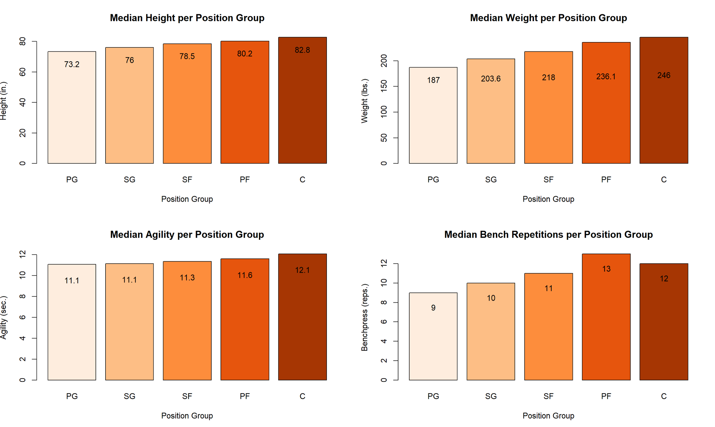
Figure 3: Median Stats per Position Group

The plot above displays the median values of 4 important physical measurements, split amongst position groups in basketball.  For reference, the positions generally scale in the direction of physically smallest to largest from PG – SG – SF – PF – C.  The bar plot results confirm this generalization as median height, weight and strength (Bench press repetitions) increase from PG to C, while agility seems to decline on the same scale. 

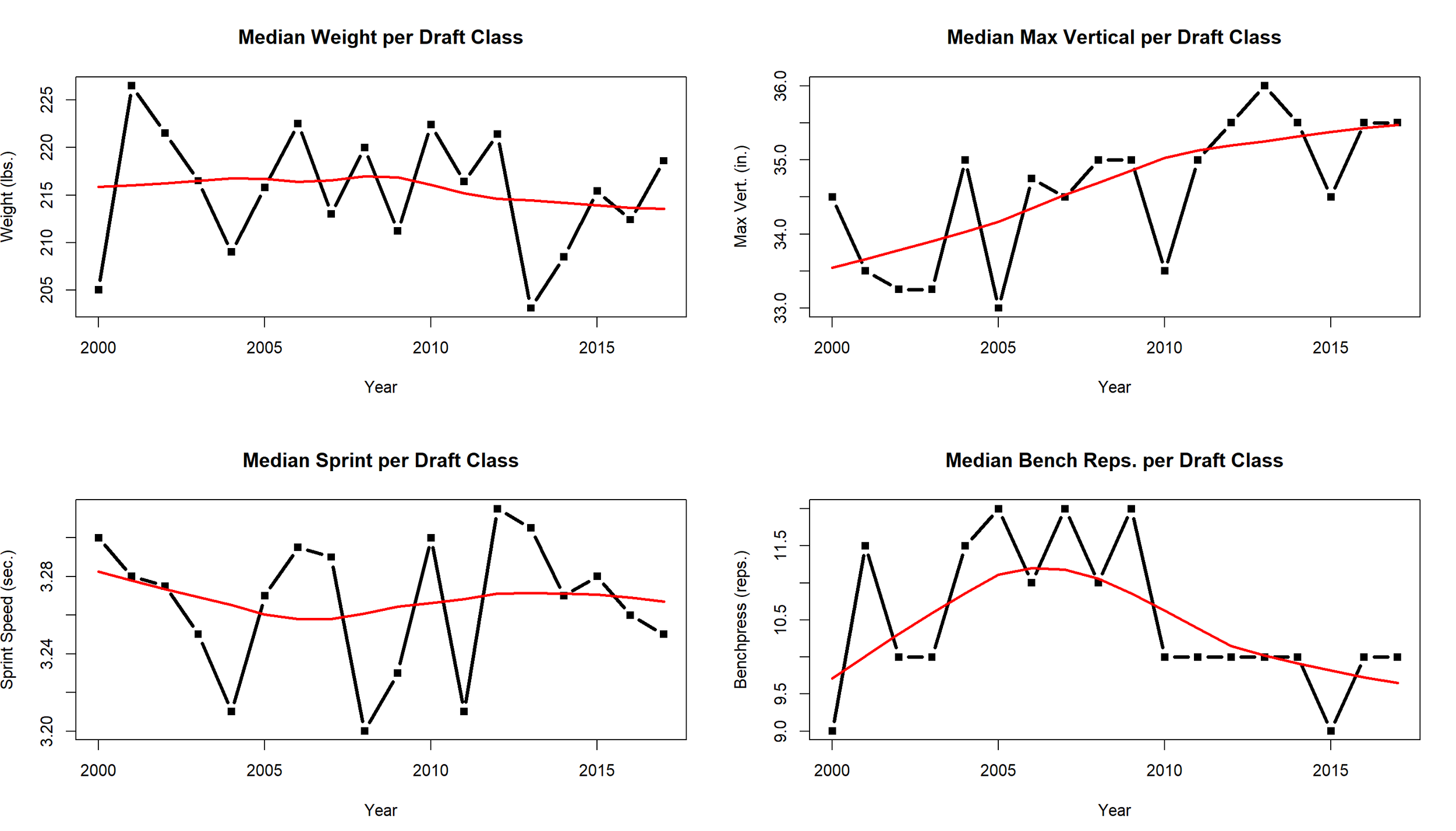
Figure 4: Median Stats per Draft Class

Figure 4 on the previous page displays similar median values but separated by each draft year, rather than player position group, to capture any trends over time.  Median weight decreases slightly from 2009 – 2017, which could coincide with a change in pace of NBA basketball which occurred around the same timeframe.  Sprint speed and bench press repetitions also showed a slight decline over this timeframe, although the bench press trend could be influenced by data imputation for the years 2014 & 2016.  The starkest increase over time belongs to max vertical leap which increased steadily from 2000 – 2017, which could signify that player candidates are increasing their verticality over time to assimilate with the pace of play or that NBA teams are increasingly placing higher value on candidates with strong verticality. Yixiong Cui noted as such in his study which identified verticality as a key measure that bifurcates NBA draftees from undrafted players (Cui, 6) Perhaps as NBA teams value verticality in their drafting decisions, player candidates have adjusted their training practices over the past two decades.

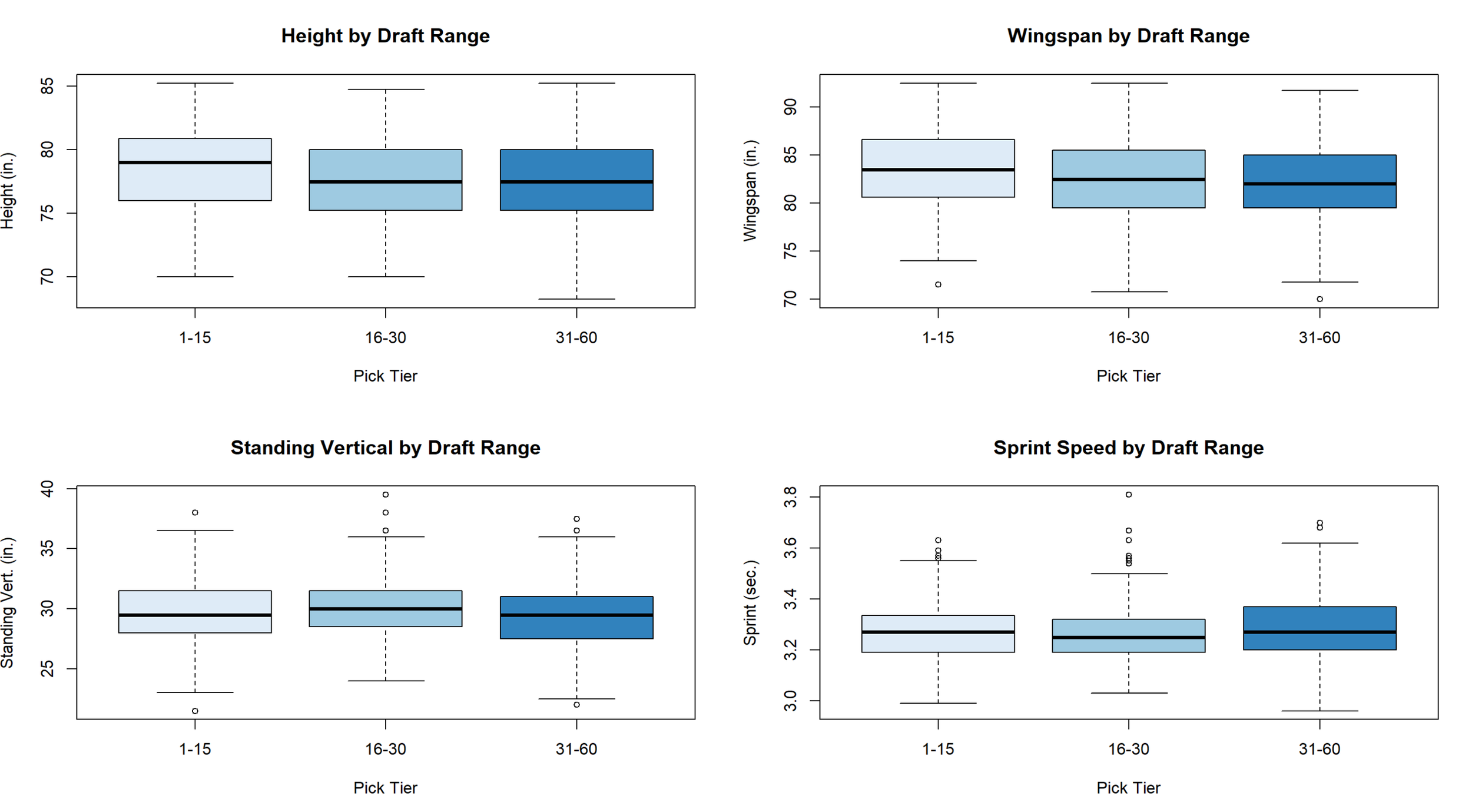
Figure 5: Distribution of Athleticism Data per Draft Pick Range

Figure 5 splits players into groups based on the position at which they were drafted into the NBA.  Lottery picks are players drafted within the first 15 picks. Picks 16-30 represent the remaining picks in the 1st round of the NBA draft and picks 31-60 represent all 2nd round picks. There are minimal differences between the groups as it pertains to vertical leap and sprint speed, but there is a slight dip across the three groups with respect to overall height and wingspan.  This could be a result of NBA teams preferring players at bigger positions at the top of the NBA draft, although it is more likely that players have slightly weaker physical measurables as the draft progresses.  These relatively small differences across draft groups further suggest that physical measurements alone may not strongly distinguish draft position.

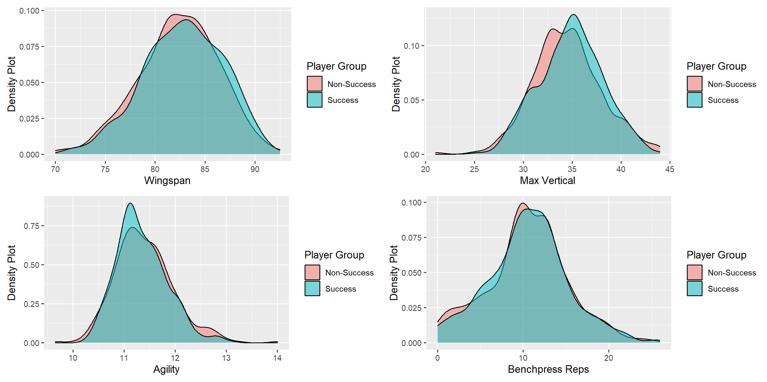
Figure 6: Density Plots of Successful vs. Non-successful NBA Players

The spread of data between successful and non-successful NBA player prospects is provided in the density plots in Figure 6 above.  Across the four athletic combine measurements shown in the above plot, there are only modest differences, with successful players exhibiting marginally higher vertical leaps and faster agility times. Otherwise, there is a significant amount of overlap across the player groups for each of the measures, indicating that, of the athletic performance data gathered at the Draft Combine, none seem to singularly separate between the two classes: successes and non-successes. This dearth of separation between classes supports the idea that a combination of variables, rather than individual metrics alone, is important in specifying a modeling approach.

Additionally, eight outliers were identified for investigation.  Through further research, it was determined that most of these outliers had a unique combination of speed and weight like Jared Sullinger – an athlete uniquely characterized by his combination of quickness and heavy weight.  Thus, these outliers were determined to be valuable for the purposes of this study and kept intact. 

A correlation heatmap showing the levels of correlation between predictors is shown in Figure 7 on the following page.  The physical measurement statistics of height, weight, wingspan and standing reach were shown to have high correlation amongst each other.  As previously mentioned, standing reach was then removed due to its high correlation with height (0.92) and wingspan (0.90) and its categorical overlap with wingspan and height.

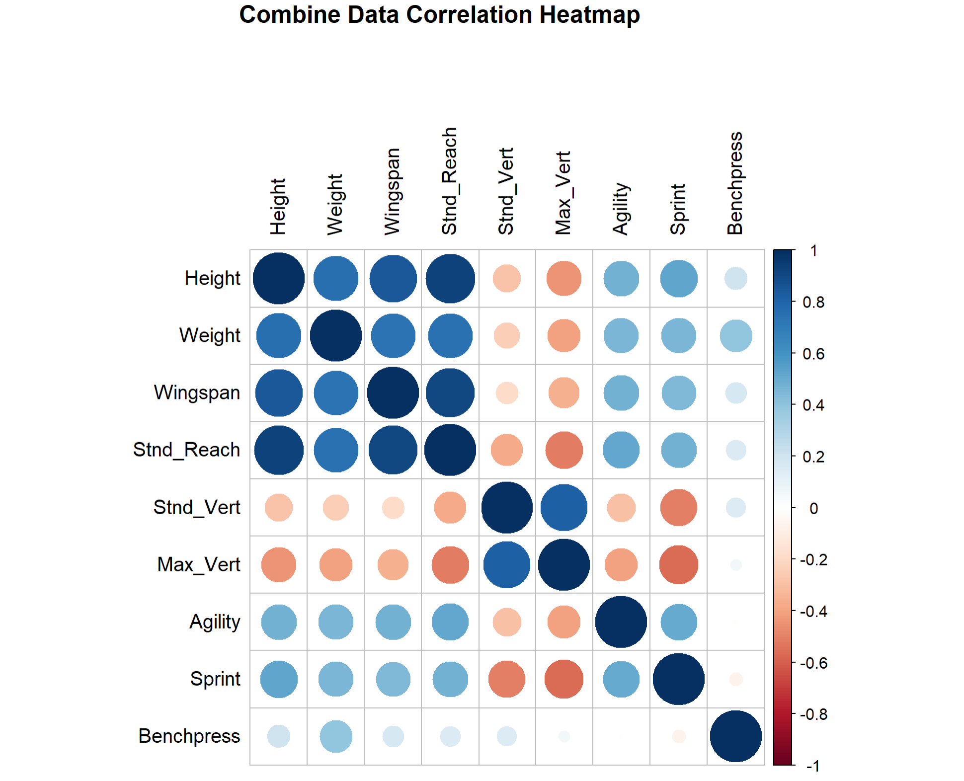
Figure 7: Correlation Heatmap of Continuous Predictors

In summation, this data exploration augments the coming prediction task by acknowledging that the variables measured at the combine elicit a limited predictive signal. The overlap of characteristics between draft pick tiers and successes vs. non-successes suggests that the variables, individually, may not offer strong predictive power and do not exhibit clear, nonlinear patterns. Thus, the use of multivariate models, described in the following section, is imperative to capture potential interactions between combine metrics.   

Proposed Methodology

The data was split using a traditional 75:25 ratio into training and testing sets. The six models listed below were fit onto the training set; and predictions were generated on the testing set. Testing error, sensitivity & specificity were used to evaluate model performance. Monte Carlo cross validation was then performed across 100 iterations to capture a more reliable estimate of prediction error by averaging testing error across 100 different splits of the data.   

Logistic Regression was chosen as the baseline classification model due to its usefulness in binary outcome prediction. A logistic regression model was fit with a binary classifier signifying a successful career as the response variable and all selected predictors as explanatory variables. This model was then reduced via stepwise regression using AIC on the training set to create a 2nd model that identifies and selects important features.   

Linear Discriminant Analysis (LDA) was included as an alternative classification approach that assumes a multivariate normal distribution and produces a linear decision boundary on which to separate successes and non-successes; LDA was chosen for a direct comparison with logistic regression, which does not provide a distributional assumption as LDA does. 

Random Forest is an ensemble method that constructs multiple independent decision trees that include bootstrap samples of the training data from a random subset of predictors. The forest model method was selected for its ability to capture interactions between variables and model potential non-linear relationships. The random forest model was fit and then tuned via the tuneRF function in R, which selected an optimal level of mtry = 4, as shown in Figure 1 in the Appendix. 

Gradient Boosting, like random forest, is an ensemble method that combines outputs from individual trees, sequentially, so as to improve iteratively upon the errors of each pre-existing model.  Gradient Boosting was included to assess whether more flexible, nonlinear modeling approaches could garner additional predictive signal beyond linear models like logistic regression and LDA. The Bernoulli distribution was specified as the loss function for this model as this study focuses on binary classification.  The tuning parameter for the optimal number of trees was decided via cross-validation on the training set, originally resulting in 161 trees out of a possible 500. Upon including Position Group as a factor, the optimal number of boosting iterations decreased substantially, from 161 to 58 (Figure 2. Appendix), indicating that Position provides meaningful predictive signal and its inclusion would benefit model performance. 

Principal Component Regression was chosen as the last model to address the multicollinearity that is present amongst the predictors related to similar athletic measurements.  Via the transformation of variables into a blend of orthogonal principal components, PCR can decrease the redundancy in the predictor set by representing the original variables as a linear combination of the predictors.  As for this study, the number of principal components in the PCR model was tuned using cross-validation, with the optimal number of components selected as four (Figure 3. Appendix), as four components is associated with the lowest Root Mean Squared Error of Prediction. Principal Component Analysis was also selected for future use in constructing a weighted composite metric to best predict which prospects will have a successful NBA career. The PCA sub-analysis is provided as an extension to the subsequent Analysis & Results section of this study.   

Analysis & Results

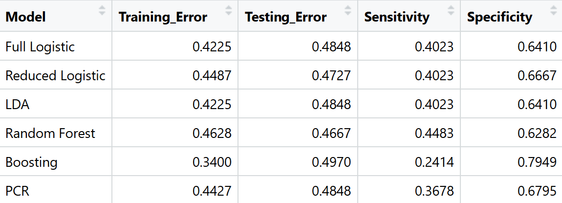
Figure 8: Evaluation Metrics of 6x Chosen Models

The full logistic regression model did not result in any statistically significant factors at the 95% confidence threshold. The reduced model with stepwise regression only kept height, max vertical, and agility as factors and had an AIC of 687.3, lower than the AIC of the full model. However, both models performed similarly with respect to testing error, suggesting that even with a simplified combination of predictors, neither logistic regression model demonstrates a strong ability to predict new data.  Additionally, the LDA model results in a testing error of 0.4848, equivalent to that of the full logistic regression model, suggesting that the multivariate distributional assumption does not improve the predictive performance of the LDA model compared with logistic regression.

The pre-tuned random forest results displayed in the left chart of Figure 9 below show the effect of permuting each predictor within a tree.  For all predictors, the mean decrease in accuracy ranges from approximately -1 to 5, which is relatively small. This suggests that the predictors do not provide much of a signal, as the removal of the most important variable, agility, would not lead to a significant decrease in accuracy. The tuned model, with mtry = 4, achieved the lowest testing error among all models at 0.4667, although the improvement over other models is slight.

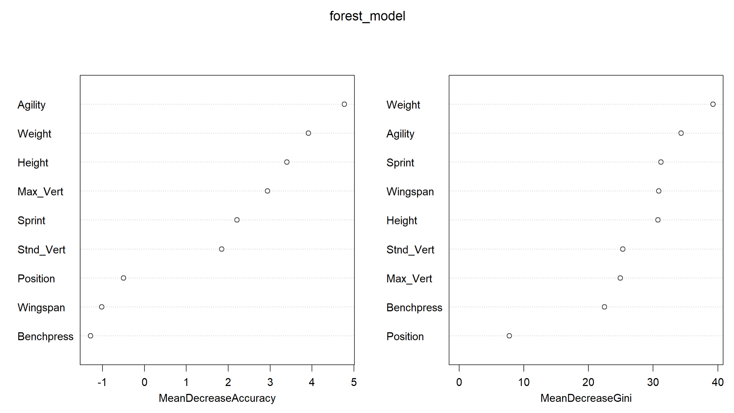
Figure 9: Random Forest Variable Mean Decrease Upon Replacement

The gradient boosting model also supports the idea that the predictors emit a weak predictive signal. Figure 2 in the Appendix shows a minimal dip in the loss function before it begins to increase, indicating that subsequent trees do not markedly improve model performance. The overall testing error is highest for Gradient Boosting at 0.4970, highlighting the weak signal and the tendency to overfit as successive trees begin to capture noise in the data. Another indication of overfitting is the disparity between the training and testing errors specific to Gradient Boosting.  The training error for Gradient Boosting is comparably low due to the model’s process of fitting residual errors and closely matching the training data. That said, due to the weak predictor signal and related noise, the model overfits the training data and offers poor predictive performance on new data. 

The PCR model offers similar results to the prior five models, as the testing error matches that of logistic regression and LDA at 0.4848. So, although the model can reduce redundancy in the predictor set and address multicollinearity, PCR did not result in any measurable improvements over the other models; this similarly indicates that the high testing errors are not primarily a result of multicollinearity, but rather weak predictor signal. 

With respect to sensitivity and specificity, all models display a significantly lower sensitivity score than specificity score, suggesting that the models are better at identifying non-successful NBA players than identifying successful NBA players. This pattern is supported by the exploratory data analysis as the density plots in Figure 6 show heavy overlap in the predictor distributions among the two classes. The Random Forest model displays the highest sensitivity score, indicating that it is the most effective model at classifying successful NBA players.  Meanwhile, Gradient Boosting has by far the lowest sensitivity score, suggesting that the model is starkly conservative in classifying a player as successful – a symptom of overfitting behavior due to weak predictive signal.

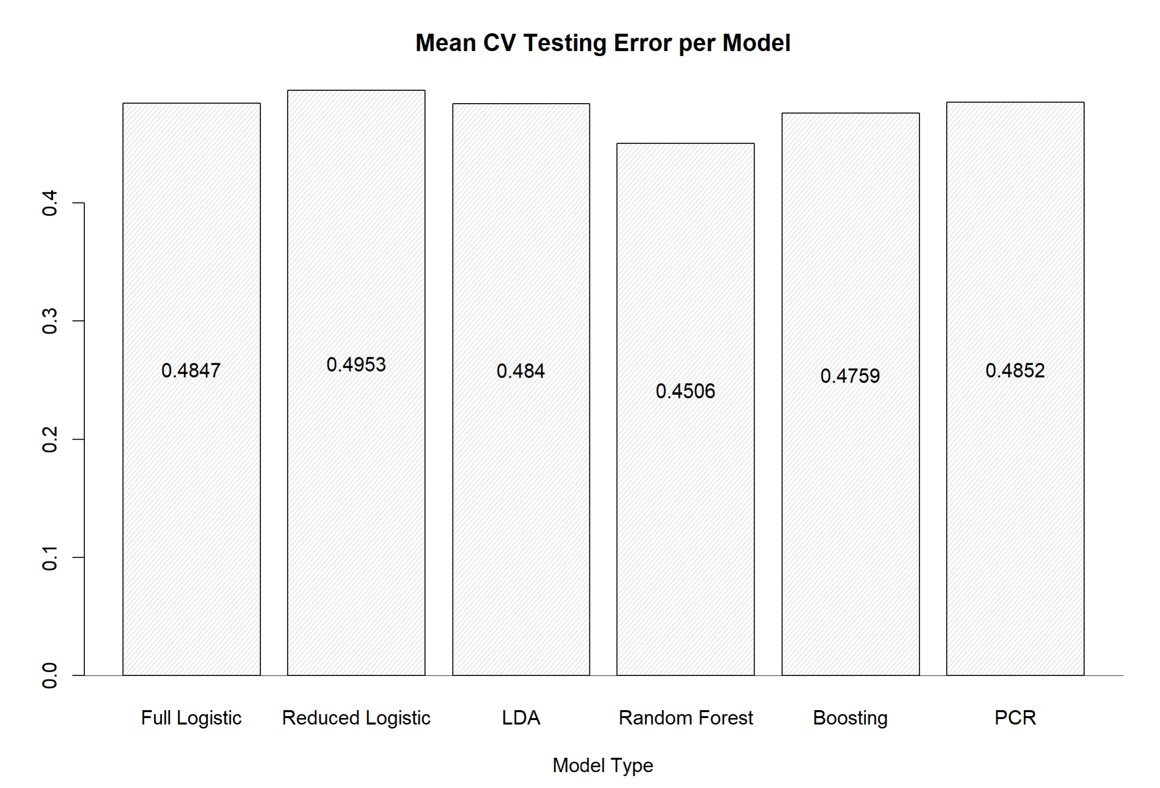
Figure 10: Mean Monte Carlo CV Testing Error 

The Mean Monte Carlo CV Testing Error results of the six models are shown in Figure 10.  Across the 100 random data splits, the CV results are similar across all models, with mean testing errors ranging from 0.4506 to 0.4953.  The Random Forest model recorded the lowest average testing error, albeit marginally, and the reduced logistic regression model recorded the highest average testing error, suggesting that selecting only the most important variables did not lead to any predictive improvements. 

A)    3x Model Testing for Frontcourt/Backcourt Split

Additional analysis was conducted by splitting the initial dataset into two position-based groups: backcourt & frontcourt.  Backcourt refers to traditionally smaller basketball players who operate further away from the basket (PG – SG) while frontcourt refers to larger players who operate closer to the basket (SF – PF – C).   Of the 662 observations in the original dataset, 288 were classified as backcourt players while 374 were designated as frontcourt players.  Each subset was then divided into training and testing sets via a 75:25 split. The proportion of successful vs. non-successful players within both groups remained balanced, thus allowing the study to proceed confidently based on the spread of response data within each subset. 

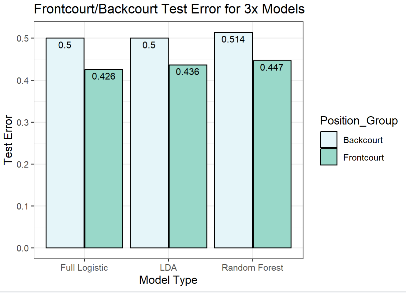
Figure 11: Test Error Comparison of Frontcourt/Backcourt for 3x Models

Figure 11 compares the testing error results across frontcourt and backcourt players for three previously implemented models: Full Logistic Regression, Linear Discriminant Analysis (LDA) & Random Forest. Full Logistic Regression acts as a baseline linear comparison, while LDA acts similarly under different distributional assumptions. Random Forest was included to capture nonlinear relationships and interaction-based effects.

Across the three models, the test error is considerably lower for frontcourt players than for backcourt players. This suggests that combine-based athletic data is more effective in distinguishing between successful and non-successful NBA players among larger athletes. This finding also implies that athletic combine measurements may be more meaningful in evaluating frontcourt prospects in the case that two prospective frontcourt players are similarly rated otherwise. In comparing the three models’ performance, Random Forest performed the worst in this position-based setting, in contrast to its performance in the earlier Monte Carlo cross-validation.  This outcome could be attributed to the decreased sample size and weaker signal within each positional group, wherein linear models would be less affected by overfitting.

B)   PCA-Based Athleticism Score

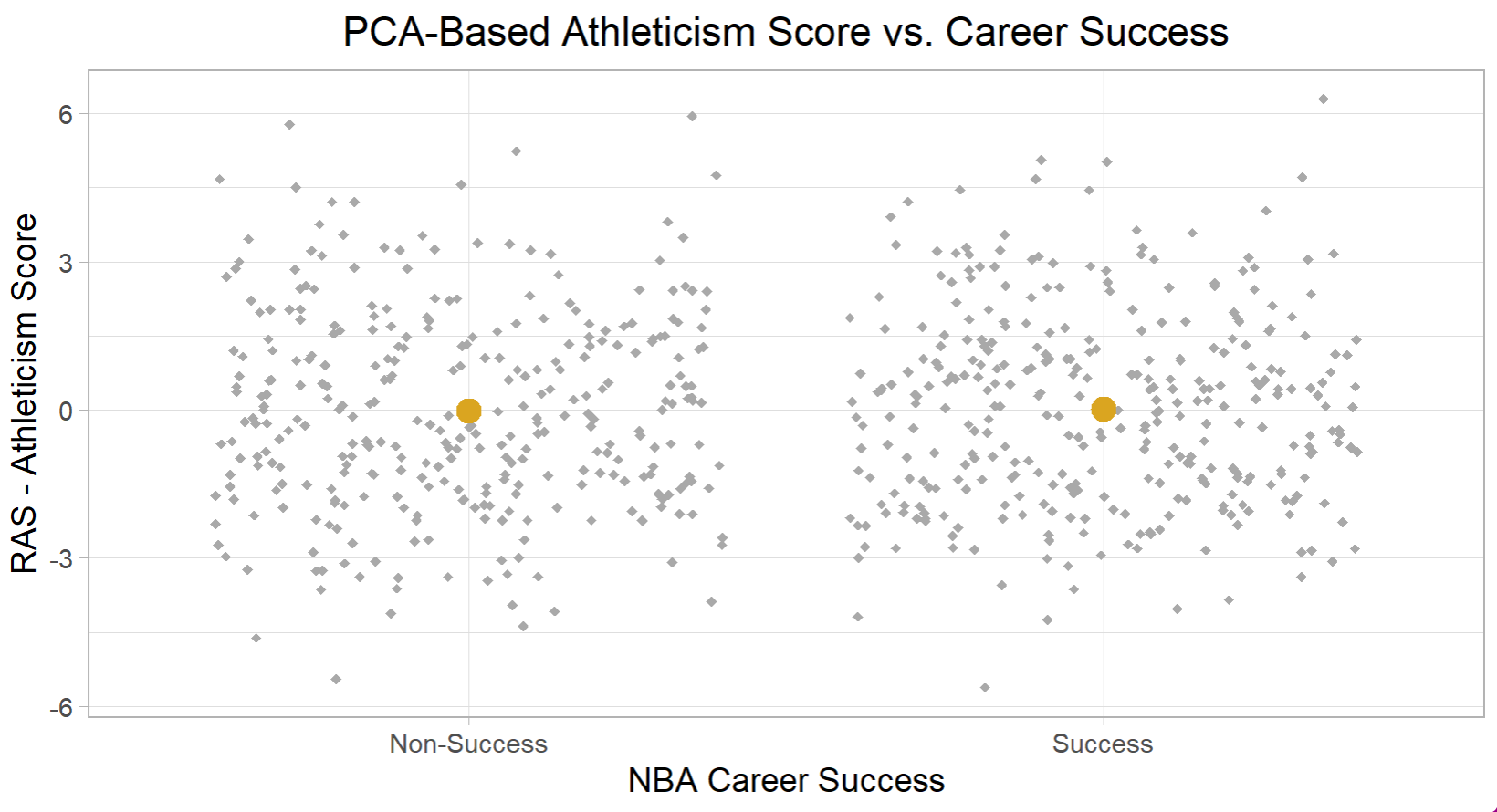
Figure 12: PCA-based Athleticism Score Comparison Between Successful & Non-successful NBA Players

In an attempt to construct an athleticism-based metric, Principal Component Analysis (PCA) was applied to the standardized combine variables, using the first principal component to generate an athleticism score similar to the RAS metric used in the National Football League. The RAS metric in this study was derived using a weighted combination of the original variables to assign a RAS value to each individual player. Figure 12 above shows the distribution of RAS scores across successful and non-successful NBA players. The spread of observations is highly similar, with mean scores that are nearly identical and centered around zero, signifying that the combination of variables into a single weighted RAS metric does not provide meaningful delineation between successful and non-successful NBA players.

Conclusions

With the given results, it is difficult to draw a strong conclusion about model performance, as the average testing errors from the Monte Carlo cross validation are quite similar across all models.  Of the predictions, the best performing model, Random Forest, misclassified 74 out of the 165 test set observations, while the worst performing model, the reduced logistic model predicted 82 incorrectly – a difference of eight predictions, which is not entirely trivial. Thus, it can be concluded that, in this setting, the Random Forest model does offer a slight improvement over the other models, likely due to how it handles interactions between weak signal predictors.

Boosting, which acts as a more computationally expensive model, does not seem to provide any improvement in prediction performance; however, the signal within the predictors is likely too weak to support any concrete conclusions. The tuning of the models did not provide any meaningful improvements, and, in most cases, resulted in slightly worse results on the test data.

Similar testing error results across all models suggest that weak predictor signal is the most likely cause for the high misclassification rate. This conclusion is further supported by the heavy overlap in predictor data in the exploratory data analysis and the small values shown in the Random Forest Variable Mean Decrease in Figure 9. Likewise, the lack of statistically significant predictors in the logistic regression and the lack of performance improvement from Gradient Boosting & Principal Component Regression suggest the same interpretation, as addressing multicollinearity and nonlinear models did not provide marked improvement. 

The PCA-based Athleticism Score also did not provide any insight into player success as the resulting distribution for successful and non-successful NBA players was nearly identical, with no discernable separation between the two groups. This outcome likewise reflects the weak predictor signal in the combine data, suggesting that a weighted composite statistic of athletic measurements does not improve the ability to predict NBA career outcomes.

Going forward, it would be prudent to gather additional data to gauge its effect on predictive accuracy, namely jump shooting data. As David Berri listed points scored, rebounds and shooting efficiency as effective measures of player value, jump shot efficiency data prior to entering the NBA is paramount. (Berri, 4) NBA players do perform shooting drills at the NBA Draft Combine in which they take the same number of jump shots at specific spots on a basketball court. That said, the data collection for jump shot efficiency is sparse and not provided on NBA websites prior to 2020. Likewise, additional datasets like collegiate or international statistics introduce inconsistencies across league, competition levels, and playing styles and are not uniformly available for all prospects. As it currently stands, although athletic combine data may be useful in comparing similarly-rated frontcourt prospects, the data alone is not sufficient in separating successful and non-successful NBA players as a whole and would be bolstered with the future inclusion of shooting accuracy data.

Credits

Several online sources, including NBA.com & The Basketball Reference, were used during data cleaning and imputation to address missing player measurements. The code for the Random Forest and Gradient Boosting sections was sourced from Statology.org.

Bibliography

a)     Kaplan, Richard A. “The NBA Luxury Tax Model: A Misguided Regulatory Regime.” Columbia Law Review, vol. 104, no. 6, 2004, pp. 1615–50. JSTOR, https://doi.org/10.2307/4099377.

b)     Xin, Lu, et al. “A CONTINUOUS-TIME STOCHASTIC BLOCK MODEL FOR BASKETBALL NETWORKS.” The Annals of Applied Statistics, vol. 11, no. 2, 2017, pp. 553–97. JSTOR, http://www.jstor.org/stable/26362197.

c)     Berri, David J. “Who Is ‘Most Valuable’? Measuring the Player’s Production of Wins in the National Basketball Association.” Managerial and Decision Economics, vol. 20, no. 8, 1999, pp. 411–27. JSTOR, http://www.jstor.org/stable/3108257.

d)     Gutiérrez, Gilberto “Performance Analysis in Basketball Players” International Journal of Sports, Exercise and Physical Education 2024, pp. 86-87. Sportsjournals, https://doi.org/10.33545/26647281.2024.v6.i1b.81

e)     Cui Y, Liu F, Bao D, Liu H, Zhang S and Gómez M-Á (2019) Key Anthropometric and Physical Determinants for Different Playing Positions During National Basketball Association Draft Combine Test. Front. Psychol. 10:2359. doi: 10.3389/fpsyg.2019.02359

Appendix

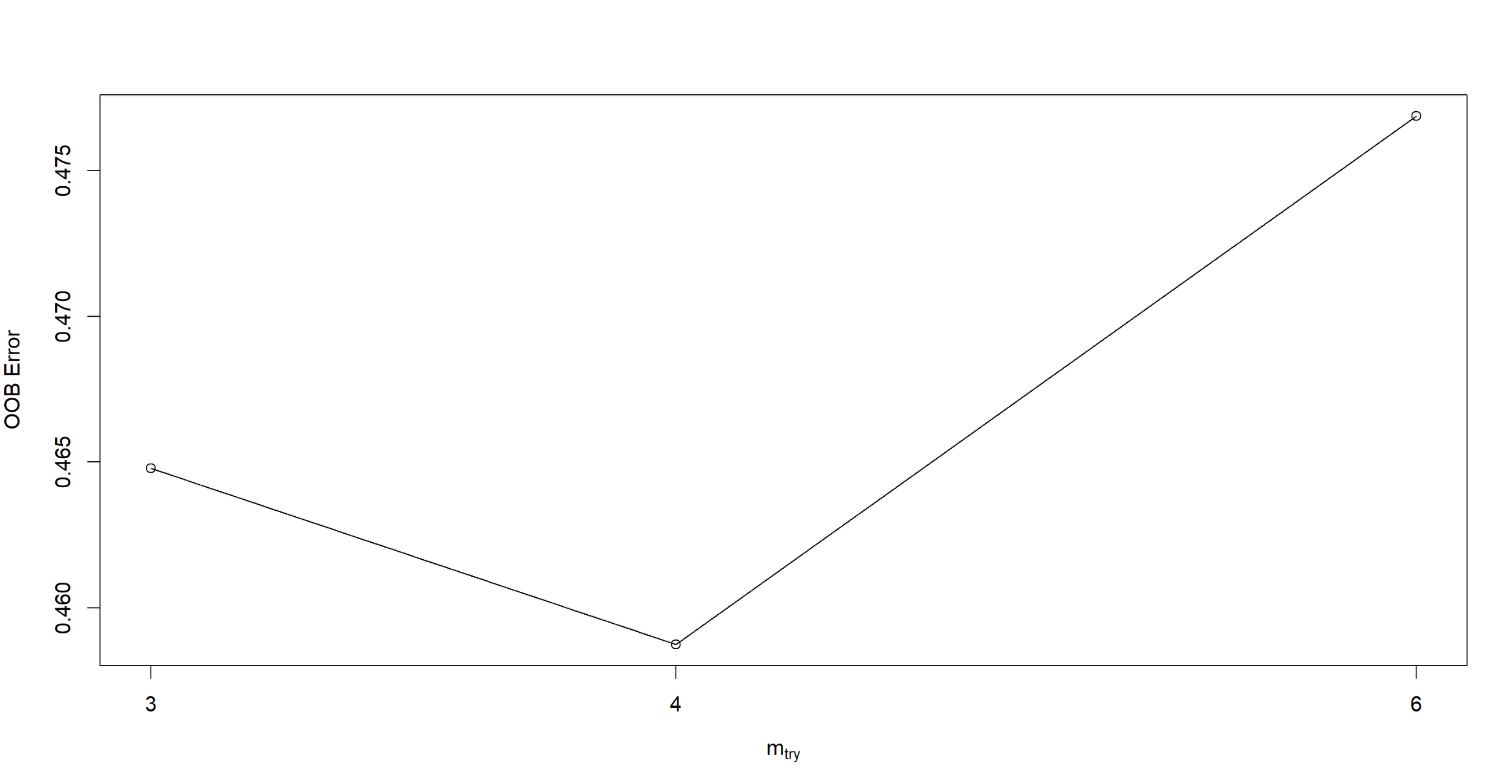
Figure 1: Forest TuneRF Function - Tuning Results

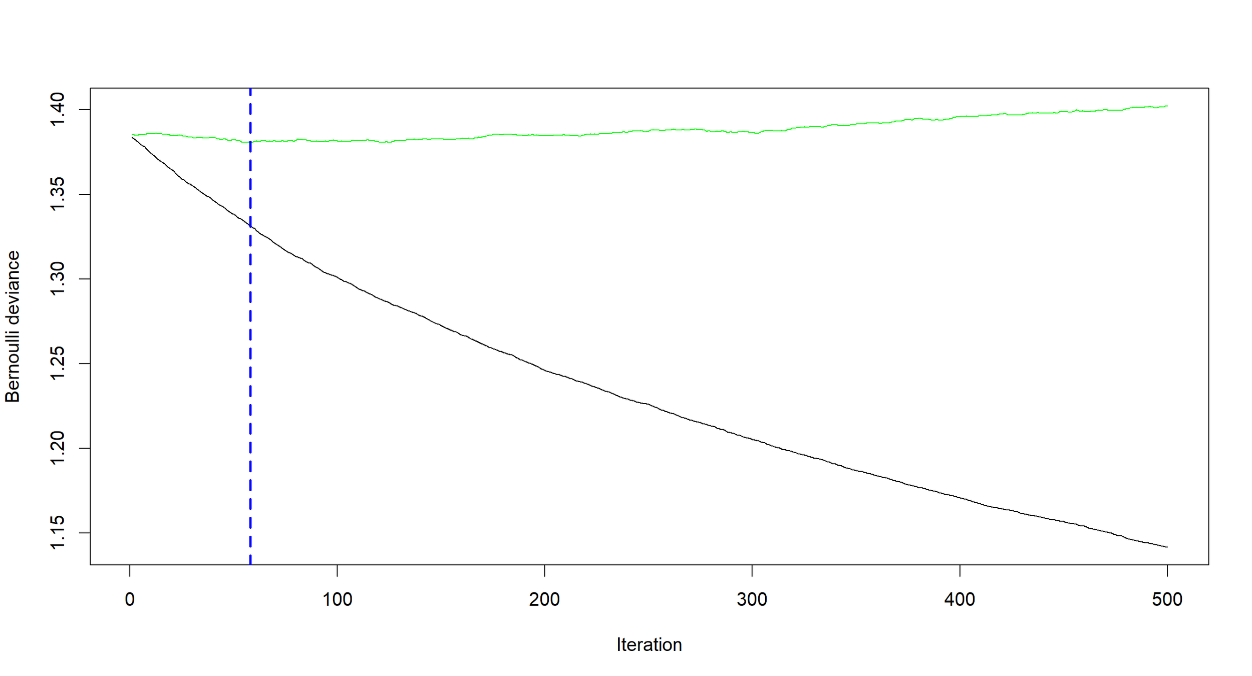
Figure 2: Optimal Tree Results from Gradient Boosting (Position included as Factor)

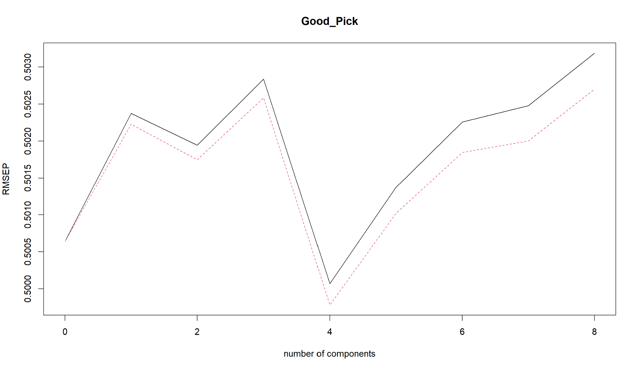
Figure 3: Principal Component Regression – Optimal Number of Components

Project Details

Methods: Logistic Regression · LDA · Random Forest · Gradient Boosting · Principal Component Regression · PCA · Monte Carlo Cross-Validation
Tools: R · RStudio