Introduction:    

In addressing rising obesity rates in the United States, I sought to understand the relationships between obesity and different socioeconomic factors: pre-existing health conditions, education level, wealth measures, and so forth. Prior research has shown that individuals with obesity are more prone to chronic conditions and require more medical visits than non-obese individuals, as demonstrated in the recent study on college-age adults (Hayes et al, 2025). Hayes’ parting suggestion that evidence-based weight management programs at universities could prove fruitful was not lost on me, as it represents a shared primary goal.  I felt that an in-depth study on several key predictors would highlight said evidence and allow for universities and locales to better conceptualize and amend their weight management programs based on which factors are most pertinent to obesity rate. 

Model/Method:

Multiple linear regression of 10 socioeconomic and health-related predictors against obesity rate was performed to assess the impact of and correlation between the 10 predictors. Additional linear models were run on alternating numbers of predictors. Lasso regression was utilized for variable selection. My initial approach here was to focus on predictor analysis and progress to more advanced predictive modeling and classification tasks in this study. 

Data:

Socioeconomic data from the CDC’s PLACES program was combined with four different datasets from the US Census Bureau for the aforementioned models: Commute, Education, Mean Income, Poverty. The merged dataset contains 67 explanatory factors, 10 of which were selected for interpretability and focus. Apart from the three variables related to Mean Income and Education, the other seven variables were carefully selected based on the limited number of existing studies dedicated to those specific factors. As studies have shown poverty level, pre-existing health conditions, and education level have a direct relationship with obesity rate, I chose to focus on mental health-related behaviors and unique socioeconomic data like the average number of vehicles per household within a ZCTA. For this statistic, I used the proportions of households with various vehicle counts ranging from 0 – 3+ and created a weighted average. This specific measure was deemed important as I sought to interpret the relationship between vehicle ownership and obesity rates. Would higher levels of vehicle ownership result in higher obesity rates because of the documented effect of income disparity?  Or is the relationship between the two variables negative due to either decreased access to fitness or a low-level city walkability index? 

Analysis:

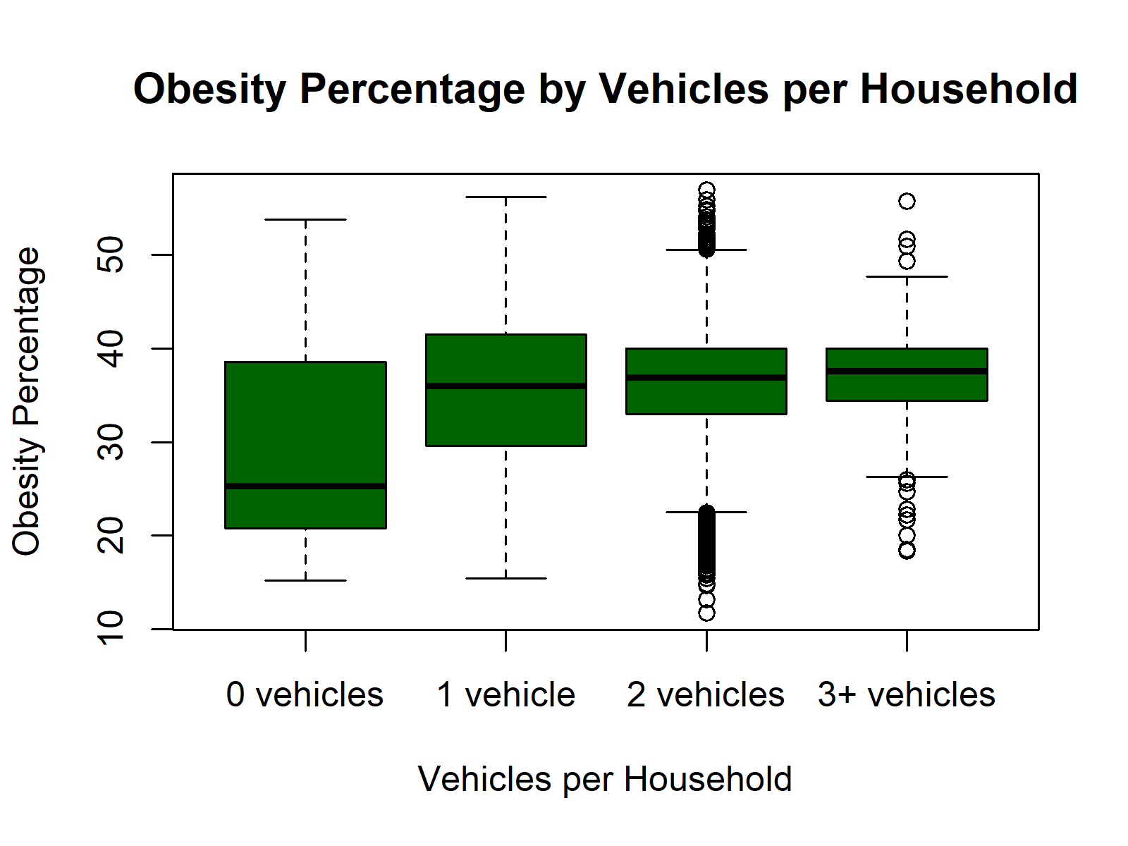
As evidenced by the boxplot, households with zero vehicles exhibit a lower median obesity rate compared to those with one, two, or three or more vehicles. There is greater variability in the interquartile range among zero-vehicle households relative to the more tightly clustered distributions of vehicle-owning households. The lower median rate for zero-vehicle households suggests that reduced obesity levels could stem from greater reliance on walking or public transportation, particularly in densely populated urban areas. The wider spread among zero-vehicle households may reflect underlying disparities, as this group likely includes individuals living below the poverty line and wealthier individuals in populated cities with extensive transit access.

The Pearson correlation matrix below further explores the association between factors by measuring the strength and direction of linear relationships. Per the graphic, the number of vehicles per household shares a positive, albeit weak correlation with obesity percentage. As for the other predictors, poverty-related measures such as mean income exhibit a strong negative relationship with obesity percentage. However, we did not anticipate that mental health-related categories like limited sleep would have as strong and positive a relationship with obesity rates. Finally, the Any Disability and Cognitive Disability predictors share a very strong correlation of 0.91, suggesting the presence of multicollinearity. 

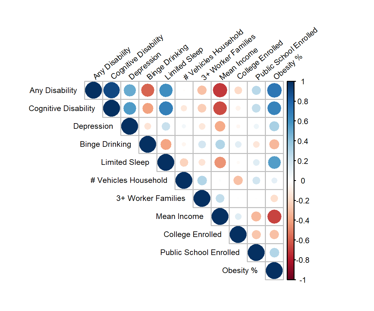
Pearson Correlation Matrix

For the initial linear model, I assessed the key assumptions, concluding from a histogram that the residuals follow a roughly normal distribution. The QQ plot also displayed linearly with a slight left-tail veering downward. The residuals vs. fitted plot does not show any non-linear patterns and assumes constant variance and linearity, though the residuals cluster around the zero line in a condensed egg or beehive shape. The bunching of residuals is likely due to how the predictors are scaled as most of the variables are percentage rates on a scale from 0-100, limiting wide variation within the residuals. Mean household income and average vehicles per household, though not in percentage form, were kept in their original form to maintain interpretability for the coefficients. 

To address potential multicollinearity, I calculated Variance Inflation Factor (VIF) scores for all predictors, targeting removal of variables with a VIF > 5. Any Disability and Cognitive Disability both exhibited high VIF values (11.2 and 9.7, respectively), indicating strong multicollinearity. I chose to remove Any Disability to retain the more focused mental health measure, as Any Disability likely captured physical comorbidities already strongly associated with obesity. Upon removal of Any Disability, Cognitive Disability no longer exhibited multicollinearity. 

Based on its high p-value (0.846) in the summary of the reduced model, the coefficient for Public School Enrolled was deemed not statistically significant.  Thus, the model was reduced a 2nd time and retrained on the remaining eight socioeconomic and health factors. Finally, a lasso regression was performed on the final eight factors to evaluate whether further variable removal could produce a more efficient model. 

Interpretation:

Under the twice-reduced model, the eight remaining predictor coefficients were all statistically significant at the 0.001 alpha level. The coefficients for Cognitive Disability and Limited Sleep highlight strong, positive associations with increased obesity rates. As expected, Mean Household Income displays a negative relationship with obesity rate. Moreover, College Enrollment, Depression and 3+ Worker Families showed negative, albeit weaker, associations with obesity rates. Binge drinking, conversely, presents a positive but weak association. Vehicles per Household, has the largest positive coefficient at 2.754, which can be interpreted as 2.754% increase in obesity percentage for every one-unit increase in vehicles per household, holding all else constant. Although the simple correlation between vehicle ownership and obesity was weak, the significance and magnitude of its impact became more prominent in the regression analysis. This phenomenon could reflect adjustments for underlying socioeconomic and health factors once the key variables were modeled together. However, the large size of the regression coefficient could partly be due to scaling differences as Vehicles per Household ranges only from 0 to 3.5, compared to the 0 to 100 scale of our percentage-based predictors. Thus, it would make sense for a one-unit increase in vehicle ownership – representative of roughly 25% of the scale range, to result in a substantial 2.75% increase in obesity rate. The adjusted R^2 decreased from 0.6651 to 0.6333 after Any Disability and Public School Enrolled were removed from the model.  Although the explanatory power of the model declined slightly after the adjustment, the lean model aligns with my goal in producing a less complex, easier to interpret model that maintains a high level of explanatory power. 

A lasso regression was run on the final model to shrink weaker predictors and reduce overfitting. Since I did not split the dataset into training and testing sets, the lasso regression was applied to the same data used for model training to get a sense of predictive ability. The lasso penalty shrank several coefficients closer to zero, especially for Mean Household Income (-5.09e-05) and 3+ Worker Families (-0.0466), which shows that these predictors had weaker influence after adjustment. Meanwhile, key factors like Cognitive Disability (0.452) and Vehicles per Household (2.705) kept relatively strong coefficients even after penalization, showing their continued importance in explaining obesity rate variation. Predictions generated from the lasso model showed that nearly all ZCTAs were predicted to have obesity rates between 20–50%. Roughly 70% of ZCTAs were in the 30% obesity range, about 20% in the 40% range, and about 10% in the 20% range. Since the predictions were made on the same data used to train the model, they don’t show how the model would perform on new data. Still, the narrow range of predicted obesity rates suggests that the lasso model was able to pick up on the main patterns in the data.

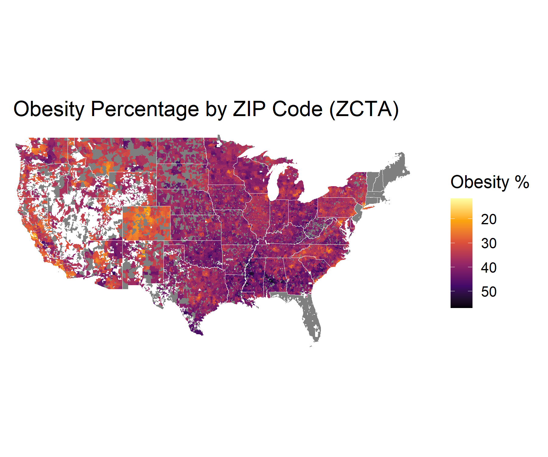
The graphic above shows obesity rates per ZCTA across the United States. Darker shades of purple represent areas with higher obesity proportions, while lighter shades of yellow represent lower proportions.  The whitespace typically corresponds to unpopulated regions, and the greyed-out sections, such as parts of the Northeast or Florida, reflect ZCTA fields with missing or non-reported data for our selected variables. Based on the output, high obesity rates appear prominent across the Central US with elevated rates throughout the Southeast, from Louisiana through South Carolina. Moving forward, my goal is to build on these findings to offer tailored guidance on weight management treatment plans across the country.  With the data from this heatmap and a deeper understanding of the key predictors that affect obesity rates, I hope to provide actionable advice on which factors are most pertinent to address within those ZCTA regions.    

Project Details

Methods: Multiple Linear Regression · Lasso Regression · Pearson Correlation · Variance Inflation Factor (VIF)
Tools: R · RStudio